ESA Easy Sky: A great tool to check the sky using different catalogs

ESA's EASY SKY

We are going to talk about an awesome tool developed by ESA that will allow us to combine in an interactive way a huge amount of images from different catalogs and missions. It will also allow us to superimpose catalogs with sources positions.

The interface is very friendly and it is quite self-explanatory:

You can find a particular source by searching its RA,DEC or provide the tool with a csv with a list of sources:

The epoch options are in the upper left part along with a popup menu that will allow you to configure what catalog images you are seeing.

A menu in the bottom part of the window will provide you with insights about how many sources you have in your fov per catalog.

This is honestly one of the coolest tools I have seen in a long time. This is the way the new astronomy tools should look like: friendly, useful, multiwavelength and combining as much catalogs as possible.

You can find the tool in the link below:

http://archives.esac.esa.int/esasky-beta/

GNSS Observables (1)

GNSS Observables (I)

There are two main measurements when it comes to GNSS observables: Pseudoranges based on the code or based on the Carrier phase measurements. At the end of the day both things are estimations of the real radial distance between the receiver and the Satellite.

To those familiar with Deep Space Operations and Navigation the closest thing to Sequential Ranging [1] in Deep Space is not the pseudorange but the carrier phase measurement in the GNSS field. The problem here is that the same ambiguities we have to face in ranging are also present here but, instead of the sequential frequency changes we have in Deep Space ranging we will have a single frequency when we measure the carrier phase in GNSS -well, we can use two frequencies, this will be useful to take the ionospheric effects out up to the 99%, avoiding the need of ionospheric models, but this will not help much with the carrier ambiguities.

Extracted from:  http://www.nasa.gov/sites/default/files/thumbnails/image/l1_dscovr_diagram.png

Therefore,  although carrier phase measurements are more accurate, at the end of the day we are using the carrier wavelength to measure the distance, this measurement will have an unknown bias due to the fact that we do not know how many cycles the carrier underwent before reaching our antenna.

When we process the output of a receiver we find measurements of both types and, depending on the receiver, at different frequencies. (When I talk about the "output of a receiver" I'm talking about a special receiver, outputting intermediate measurements not the typical Position Velocity and Time (PVT) final measurement. Luckily a RINEX formated file with these measurements).

Therefore we should keep in mind that when we look into Carrier phase measurements we are dealing with an accurate measurement but biased by an entire number of cycles. An entire number that will also change as soon as the receiver gets out of lock, so you should expect bumps in the data.

Following picture shows real GPS carrier (Lx) and pseudorange measurements (Px and Cx). As you can see the distance difference is huge. We know GPS Satellites are placed in MEO orbits so we should expect measurements around 20000 Km. Therefore we know for sure carrier phase measurements are biased.

We will keep talking about GNSS observables and how these measurements are done in following blog entries, stick around!

===========================================================

[1] Deep Space Ranging http://trs-new.jpl.nasa.gov/dspace/bitstream/2014/40972/1/07-0166.pdf

Delta DOR (This is a different approach to ranging and will provide us with angular measurements (not the distance to the satellite) and combines VLBI measurements. Nonetheless I think these slides are quite good to have some insights on Deep Space Navigation) http://www.slideshare.net/esaops/ops-forum-esa-delta-dor-from-implementation-to-operation-16032007

[Easy trick] Data Joy. Google Drive for coding.

[Easy Trick] Data Joy. Google Drive for coding.

Some months ago I found a company offering a very cool tool for coding purposes. What if you could work on your coding projects in the same way you do it in Google Docs? What if you could chat and work on the same code in group? What about also being able to test the code online?

This is exactly what DataJoy offers to you: an online tool that allows a group of people to work on the same code in real time, with chat features and allowing you to execute your code obtaining the stdout of your code or even graphs directly in your web browser!

You can upload your current python code, csv files... it is full of features so keep an eye on this tool!

Do not hesitte and check it out now!

[Easy trick] Examine an entire directory tree using python

[Easy trick] How to easily analyze an entire directory tree: os.walk

Today we are going to talk about a small problem you sometimes have to deal with: evaluating an entire directory tree in order to find some types of files. Say that the user is manually leaving these files at random places (very typical), that you want to make sure you are not missing a particular file or that you want to know some folders size (sometimes Linux does not show you the size of a folder but the size of a the file representing the folder (4096 bytes), therefore creating a script to evaluate what is the bigger folder in, for instance, a project directory tree is quite straightforward).
The "os" python library has a very nice method called "walk" that will return an iterator you can use to obtain all files names.
We should provide os.walk() with a string indicating what folder we want to "walk" trough.

This option for instance will provide us with an iterator with all the subdirectories from /.

You can even obtain folder, files and the folder names that being evaluated (root)

This is an easy trick that is very useful for many applications.

If you want to go downto a particular subdirectory you should recurrent calls of this method.

JPL Spice in Python

Dealing with Deep Space Spacecrafts orbits: JPL Spice

In this blog entry I am going to talk about the JPL Spice toolkit and how to use it for calculating signal parameters for a real Deep Space Spacecraft.

The JPL Spice toolkit is cool tool that allows us to calculate positions and velocities (the complete state vector) between two objects in the Solar System. It also allows us to see whether a particular FOV (Field of View) of a spacecraft instrument is going to cross the surface of a planet, a moon or any other thing, and when that is going to happen. In Spice there are two well differentiated things: one is the observer and the other one is the target. Nonetheless they are intercambiable, an object can act as the observer or as the target.

JPL uses this tool for mission planification or while using the data obtained by a particular instrument (there is also a standard for archives that takes into account this info, the ancillary data).

In order to provide the Spice library with the necessary data we should load in its pool the files with data about the spacecraft, satellites, receiving station... whatever we need to sort out our problem... These files with data are called Kernels. We have Binary kernels and ASCII kernels. Kernel formats are well documented in the NAIF webpage (NAIF is the department in charge of SPICE in JPL).

There is a very nice training in the NAIF webpage that could be of interest for you if you want to develop your own application. As for now (October 2015) JPL Spice supports Matlab, C, Fortran and IDL.There is a non-official version of Spice for Python, called SpiceyPy, this is the one we are going to use in our examples.

The problem we want to sort out

Extracted form NAIF tutorials

In order to extract details on how we are going to receive the spacecraft signal on Earth we need first to properly understand the Solar System geometry and some timing considerations we have to take into account.

• Geometrical Considerations: The first thing we should take into account is that we need to know what is the reference frame of interest for each object. Say that you know where your Ground Station is located, for instance the NASA Madrid Deep Space Communication Complex, particularly the DSS-63 antenna, which is 70 meters in diameter. We know that this antenna is located, assuming the Earth is an sphere - if you need more accuracy you should use  kernels with the necessary data about the DSN stations in a topocentric reference frame. You can check here what these kernels look like-, at (4º 14' 53'' 40º 25' 54'') [Don't use these values as I think it points to the middle of the MDSCC not the accurate position of DSS-63].  In this case you have the position of the antenna referenced to the Earth, and you need to know where is the Earth referenced to the Solar System Barycenter (SSB), and also where is your spacecraft... and your spacecraft will probably be referenced to the body it is orbiting (or not) so you will need to know where that body is located referenced to the SSB... all this data should be provided to Spice by means of Kernels. It is not clear in the latter figure but the center of the J2000 reference frame should be located at the SSB.
• Timing considerations: Once we have sorted out the geometrical problem, we should address the following and very connected problem: time. We need to know the position of all these objects in the same time span or we will not be able to determine a single thing. In fact this is one of the most typical problems you will face: you are loading kernels that are not covering the same time span. Check the kernels headers to ensure proper timing alignment. Now, once we said that, you will need to provide following kernels to relate a UTC time on Earth to time in a spacecraft: Leap Second Kernels (LSK) and Spacecraft Clock Kernels (SCK). Leap Seconds Kernels will provide us with the Leap seconds added or substracted during the last few years and future planned Leap Seconds (allowing converting time from UTC to Ephemeris Time (ET)) and SCK Kernels will provide us with data about the Spacecraft atomic clock (a spacecraft could have more than one clock), providing us with details about the clock status and performance. This will allow us to convert from Ephemeris Time to Clock Time ("Ticks" which is the smallest increment of time that a spacecraft clock measures).

Kernels:

Let's review some of the Kernels we have available to perform our calculations.

• SPK : This Binary Kernels will provide us with data about the orbit of an object relative to something (eg: Cassini relative to Saturn Barycenter). The way orbits are described in these files is important depending on the problem you want to sort out. Positions and/or Speed could be described in different ways in the SPK Kernels: as modified divided difference arrays, Chebyshev polynomials, weighted two-body extrapolation, Lagrange interpolation... If you want further details on SPK types please check this pdf.
• TLS: As mentioned before this ASCII Kernels provides us with a yearly tabulated list of added or subtracted leap seconds. Past or programmed for coming years.
• CK: Known as Orientation or Attitude Kernels. These Kernels will provide us with details on the orientation of an entire spacecraft or parts of the Spacecraft structure. It contains information about rotations referenced to a Reference Frame. We can use these Kernels to learn the orientation of a spacecraft instrument that will help us to know, once we know where our Spacecraft is located, whether our instrument is going to point to an interesting object or not for a particular instant. As in the case of SPKs there are different ways of detailing this data. For further information on CK types please check this pdf out.
• IK:  Instrument Kernels. In the latter type of kernel we were talking about knowing when our instrument will be able to "see" an object depending on Spacecraft position, object position (maybe even object orientation) and instrument orientation. But one point was missing: We need to know and to model the Spacecraft field of view (FOV). Without that information we would not be able to accurately model what our instrument is going to be able to see. Therefore specifications for FOV size, shape, and orientation are contained in these files, it could also contain internal instrument timing and calibration data.
• FK: Reference Frame Kernel. Spice Supports inertial (fixed) and non-inertial (non-fixed) reference frames. Some of them are built-in, like the J2000 (Z normal to the mean Earth equator at J2000 epoch, please also note that in SPICE ICRF=J2000 Reference Frame) and some others could be loaded using these Kernels.  
• PCK: Planetary Constants Kernels. These Kernels could contain binary or ASCII data. These Kernels contain generic details on SS bodies like orientation or shape. In some cases polynomials are used to model the pole position. Bodies high accuracy orientation is stored in binary PCKs.
• Meta Kernels: These Kernels could be defined as similar to headers files in C. It just allows you to import a large list of kernels just by asking in your code to load a single. You can find these Kernels syntax in the Spice tutorials. If you are planning to use a large number of kernels you should use them.
• Transaction Kernels: These ASCII Kernels are just ASCII representation of binary kernels. The extension is the same of the binary one but the first letter is changed by a "x": .x*. By the way: be careful with ASCII Kernels and the editor you use while editing them as some invisible ASCII characters may be included in the document that may make Spice to not being able to process the Kernel. For binary Kernels make sure you have a clear idea about endianess and so on.

Example 1: Cassini Orbit around Saturn. In this easy example we are going to see the orbit of Cassini Spacecraft around Saturn Barycenter using Python. This is a classical example.

You can find the code in Github.

Example 2: Doppler influence due to movement between Earth and Cassini. We are going to calculate the Doppler influence due to the relative movement between Cassini and a Earth Ground Station at the Madrid Deep Space Communication Complex.

You can find the code in Github.

You will need the meta kernel and also to download the necessary extra kernels.

Web Geo Calc (WGC):

You can check that your program is performing well by using the WebGeoCalc tool of JPL.

It is very easy to use compared to coding your own application. Nonetheless there is also a tutorial on this.

Parabolic frequency estimator.

Parabolic frequency estimator.

This is an interesting problem. Say that you have a DSP (Digital Signal Processing) system implemented, for instance in an FPGA, say that you have a tone in a particular frequency and you want to know exactly what is the frequency of your tone.

So, what do you do? Well, you just find the maximum in your spectrum and then see what is the frequency bin where your tone is located (suppose you have a clean spectrum). If you are using the typical FFT Xilinx core you will have two very useful outputs of the core that you can easily use to implement implement the "search for the maximum" algorithm with some extra effort. So far so good, right?

But there is something you should take into account: The spectral accuracy you have there. That bin, where your maximum is located (by the way, think about what is going to happen if your tone falls just in the middle between two different bins. And if you are thinking that you are designing your system to avoid this problem, then think about doppler frequency shifts if you are working with a moving receiver or transmitter (eg: a spacecraft)... you will have to implement a low pass filter in your maximum bin finder).

That maximum bin you found will not provide you with the exact frequency, say you calculated your FFT with a 1024 points accuracy. You already know our frequency resolution will be fs/N, where N is the number of points you used to calculate your FFT.

Is it a problem? Absolutely and, as we are going to see in the next few minutes, results can vary significantly due to this problem (how significantly will depend on the system and its importance will depend on exactly the same thing: your system design and application). In order to check whether that is true or not we will use a Python program that will extract maximum directly from the bin finder and will also use a frequency estimator, particularly a parabolic estimator.
All the blog entry and the program is based on this paper:

http://www.eee.metu.edu.tr/~ccandan/pub_dir/FineDopplerEst_IEEE_SPL_June2011.pdf

There is cool mathematical explanation in this paper which is interesting to read. If you have a clean spectrum then, after calculating your spectrum and finding the maximum bin, then you calculate:

Where:

This will help us to find the real maximum value. In DSP system where knowing the exact frequency is very important this could be very useful.

You can extract a simple (very simple) code that demonstrates the parabolic estimator, here:

https://github.com/fgallardo/sandbox/blob/master/freq_estimator.py

Let's take for instance a frequency value of 1KHz and we want to estimate it with a 1024 points FFT.

##########################################
This is the frequency estimated with this method:
1000.09993501 Hz
This is the real frequency the sinusoid have
1000 Hz
This would be the value we would have with a spectral resolution of 1024 points:
996 HZ
#########################################

Therefore by using our FFT with 1024 points we would end up by estimating that our frequency was 996Hz and it turned out it wasn't. We had a 0.4% of error, by estimating a frequency 4Hz under the real value.

This is an interesting point to take into account while working on our DSP systems.

Take care!

Non-equal smapling. Lomb-Scargle spectrogram.

One of the most typical problems you face when you are trying to find periodicities in astronomical time series data is the sampling period. You may think (and if you’re a telecommunications engineer as I am, I bet you directly thought about it) about using the Fast Fourier Transform (FFT) or the DFT.

You can try that and you may obtain results that could be valid… or not. Especially if you are willing to analyze data in an iterative approach then you should not do this as you may end up facing a problem with some of your results (at least check the sample time in provided data).

Let’s take for instance this case: a file with magnitude time series data of a Cepheid star. As you may know you can use these stars as standard candles for some range of distances, Henrietta Leavitt realized in 1912 that there is a relationship between the periodicity of these stars and their luminosity. Therefore we can use this relationship to calculate the distance to a star. More about the method here.

You can use any program you want to perform the FFT or DFT on the time series data, for instance Period04, which is a cool Java program that you may want to use for analyzing data (it could be helpful for some simple analysis about periodicities and could be used for prewhitening processes in asterosismology).

You can find Period04 program  here.

So, if you analyze this data using Period04 you will end up having this spectrum:

Where you can easily see that the main periodicity is located at 0.42 cycles/day (BTW: another note for engineers, as samples are taken on nearly daily basis we will not be talking about Hz but c/d).

Well, you may think this is the way it is supposed to be… not so fast. Something I learnt while analyzing this type of data: mind the time axis, mate… The first tip you should extract from here is: don’t try to analyze something you don’t really understand: how was your data captured? What is it representing? And especially: is the sample time constant? If your background is electronics and DSP related, then you may be used to have a constant sample time. Forget about that. That may be true here but is not always true. 

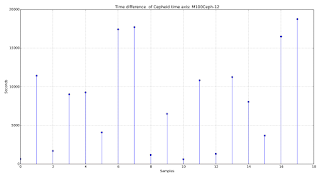
First thing first, let’s see what is the time difference between each sample. You can do it in matlab or python by using diff. If you are using python just import numpy (import numpy) and then use numpy.diff on your time data. These functions calculate something similar to the derivative, it just takes each sample and subtracts them one by one Therefore this will give us the difference between each sample. If you are not very familiar with Python then you will find an example about this at the end of this article. If you are used to code in Python then you will find this very very easy.

As we can see there is a huge difference in the sample time value. We should not use this particular method for analyzing this data. So, what can we use?
Well, there is a nice periodogram called the Lomb-Scargle periodogram that will allow us to compute the spectrum of our time series but accepting these irregularities we saw in the sample time values.

This periodogram accept time lags in the basis functions it uses for projecting our data and searches for the best solution. We will be obtaining the most accurate spectrum by using this technique. Therefore forget about using FFT in this case and use this spectrogram, it could be slower but you will obtain a more accurate result.

 Where Tau is the supported lag that will be used to make a least-square fit to maximize the orthogonality of both basis functions.

Ok then. Let’s use it!

You can find a nice implementation of this periodogram in Python here.

The way of using it is (again: if you are not used to code in Python then you will find an example at the end of this article on how to use it and some data to test it) you should import the Lomb-Scargle periodogram before using it. If you placed the periodogram python code in the same directory then just do “import lomb” and we will be ready to go.

Now we should use this function call lomb.fasper(time_value, magnitudes_value, oversampling, Nyquist_freq)). Be aware that you should provide the function with the following parameters: times vector, magnitude values, the oversampling factor, and a factor that will be use to analyze up to Nyquist_freq*factor frequency.

The result is the following:

 As you can see it is different. It turns out the that most important periodicity in this time series was not the one at 0.42 c/d but 0.047 c/d.

I hope this may help somebody trying to deal with this particular problem.

Take care!

Cepheids data: https://drive.google.com/file/d/0B3aZza3bav9gODBFR3VoQm04LWs/view?usp=sharing

PS: I prepared a cool Latex entry but it seems to have a huge amount of compatibility issues with blogger, I'm afraid format is quite poor. :-(

----------------------------


#!/usr/bin/python
import numpy as np
import matplotlib.pyplot as plt
import csv
import lomb

def proce(tipo):
    names=list()
    salida=list()
    auxi=list()
    for z in range(12):
        aux=list()
        if z+1<=9:
            nombre="M100Ceph-"+'0'+str((z+1))+".txt"
        else:
            nombre="M100Ceph-"+str((z+1))+".txt"
        names.append(nombre)
        f=open(nombre,"rb")
        k=csv.reader(f,delimiter="\t")
        for row in k:
            for z in row:
                auxi.append(float(z))
            aux.append(auxi)
            auxi=list()
        salida.append(np.array(aux))
    domin=1 #Just change it if you want to see time domain signal
    if tipo==1:
        for k in range(len(salida)):

            
            t=salida[k][:,0]
            y=salida[k][:,1]

            ##---------
            #Plotting time difference
            plt.figure()
            plt.stem(3600.0*np.diff(t))
            plt.xlabel("Samples")
            plt.ylabel("Seconds")
            plt.title("Time difference  of Cepheid time axis: "\
                +names[k][0:len(names[k])-4])
            plt.grid()
            #---------
            plt.figure()
            if domin==1:
                fs=(1/np.diff(salida[k][:,0]).max())
                FOUR=salida[k][:,1]-(salida[k][:,1].mean())
                Pun=len(y)
                t,y, nout, jmax, prob = lomb.fasper(t,y, 6., 6.)
                #print (prob)
                print (salida[k][:,1].mean())
                #y=y*y.conj()
                plt.xlabel("Frequency (c/d)")
                            
            
            plt.ylabel("Magnitude")
            plt.plot(t,y)
            if domin==0:
                plt.xlabel("Days")
                plt.gca().invert_yaxis()
            if domin==1:
                plt.title("Lomb-Scargle periodogram  of Cepheid: "\
                +names[k][0:len(names[k])-4])
            else:
                plt.title(names[k][0:len(names[k])-4])            
            plt.grid()
            
        plt.show()


    return np.array(salida)    


if __name__ == "__main__":
    proce(1)